How NVIDIA Cosmos 3 and SageMaker HyperPod Power a Physical AI Model Factory

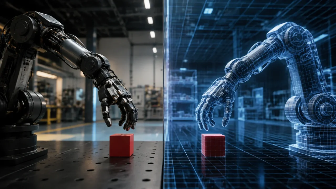
Building a robot or autonomous vehicle is not a one-job training problem. It is an operating loop: collect and curate real-world observations, generate synthetic examples, post-train perception and policy models, test those models in closed-loop simulation, deploy them, capture new failures, and begin again. AWS describes this continuous system as a Physical AI model factory.

The proposed implementation combines NVIDIA Cosmos 3 with Amazon SageMaker HyperPod orchestrated by Amazon EKS. Its defining infrastructure choice is to place generation, training, and evaluation on one persistent GPU pool connected to one shared storage layer. That avoids creating and dismantling separate environments for every stage, while keeping data and checkpoints close to the workloads that consume them.

This changes the performance question. When GPU capacity is committed for an entire campaign or reserved indefinitely, the most important metric is not the fastest isolated training step. It is GPU goodput: useful progress across the complete pipeline per reserved GPU-hour.

How Cosmos 3 supports the factory

Cosmos 3 is an omnimodal world foundation model that handles video, images, actions, and sound in one token stream. Instead of attaching a diffusion video generator to a separate vision-language model only at the end, it integrates reasoning and generation throughout the transformer trunk.

Three design choices enable this arrangement:

• A shared sequence: Text and vision inputs occupy an autoregressive region, while generated video, audio, and action tokens occupy a diffusion region. A vision transformer handles image understanding, and a frozen Wan2.2 video variational autoencoder handles pixel generation.
• Two experts at every layer: A reasoner predicts the next token while a generator denoises video, audio, and actions. Dual-stream attention connects them layer by layer. Diffusion queries can attend to both autoregressive and diffusion keys, while autoregressive queries remain causal and cannot see the diffusion tokens.
• Different training and inference workloads: Training executes the complete denoising schedule and decodes video because predicted video contributes to the loss. Robot inference uses only a few denoising steps and skips video decoding. Video latents still help ground the action, but only action tokens become executable joint positions.

Three action modes, one architecture

The base checkpoint changes roles according to which tokens begin as clean inputs and which begin as noise. In forward dynamics, the action and present frame are known while future video is denoised, making this the synthetic-data mode. In inverse dynamics, video is known and actions are denoised, allowing unlabeled recordings to become action-labeled data. In policy mode, action and future-video representations are noisy; the model conditions on a three-view image and proprioception and predicts 32 future joint positions.

Cosmos3-Nano has 16 billion parameters and uses a dense 8 billion-parameter Qwen3-VL backbone. Cosmos3-Super has 64 billion parameters on a dense 32 billion-parameter Qwen3-VL backbone. Cosmos3-Edge is a separate 4 billion-parameter tier built on a roughly 2 billion-parameter backbone trained from scratch. Because Edge has a distinct weight lineage, it is post-trained directly for target hardware rather than obtained by shrinking Nano. The DROID policy variant operates at 15 Hz with a 32-step horizon. NVIDIA released Cosmos 3 under the Linux Foundation’s OpenMDW-1.1 license.

From a model to a continuous flywheel

The model factory has four recurring stages. First, DROID, BridgeData2, autonomous-vehicle sensor logs, or other real-world data are curated into a shared corpus on Amazon S3 and Amazon FSx for Lustre. Second, a Cosmos3-Super teacher generates synthetic material. Third, the combined corpus post-trains a deployable Cosmos3-Nano policy while vision fine-tuning can span Nano and Super. Fourth, closed-loop simulation evaluates the policy, and observed failures become targets for the next generation round.

HyperPod maps that flywheel onto a persistent EKS control plane. Generation runs through vLLM-Omni, post-training uses cosmos-framework under torchrun with FSDP2 and Ulysses context parallelism, and evaluation uses a single-GPU policy server. All three mount the same FSx for Lustre namespace, backed by S3 through a data repository association. Synthetic clips, datasets, and checkpoints consequently remain available without terabyte-scale transfers between clusters.

HyperPod also monitors nodes, reboots or replaces faulty instances, and can recreate the PyTorchJob pod group. NCCL then reforms the distributed process group, while cosmos-framework resumes from the latest PyTorch Distributed Checkpoint. The maximum duplicated training work is bounded by the checkpoint interval, plus replacement and scheduling latency.

Optional task governance, built on Kueue, can divide shared capacity into namespace-scoped queues with quotas, priorities, and preemption. It is unnecessary for a single embodiment but useful when many robot or vehicle projects compete for one reservation. Conversely, a small, one-off fine-tune may be better served by an ephemeral managed training job; the persistent HyperPod design is aimed at continuous generation, long multi-node runs, shared evaluation, and scales where failures become more frequent.

The three representative workloads

AWS exercised three workloads with real checkpoints on p5en.48xlarge nodes, each containing eight NVIDIA H200 GPUs:

• A Cosmos3-Nano robot policy trained on a public LeRobot v3 DROID dataset, representing the lightest per-step workload.
• Cosmos3-Nano supervised vision fine-tuning on video-caption data, with substantially more work per step.
• Cosmos3-Super vision LoRA fine-tuning with context parallelism, the heaviest workload.

The source does not demonstrate autonomous-vehicle post-training directly. It notes that the base models used the public SDG-DriveSim synthetic-driving corpus and that the per-embodiment action projection is designed to support an AV ego-pose action space. That makes AV use an extension of the recipe, not a result established by the walkthrough.

Preparing the HyperPod EKS cluster

Prerequisites and health controls

The environment requires an EKS-orchestrated HyperPod cluster, p5en.48xlarge nodes in one Availability Zone, sufficient regional service quota, kubectl, the Kubeflow Training Operator, the FSx for Lustre CSI driver, and an FSx filesystem in the same VPC and subnet as the GPU nodes. GPU availability is a binding constraint, so the source recommends arranging a flexible training plan or capacity reservation rather than assuming on-demand p5en supply.

Generation and policy serving also require a Hugging Face read token whose account has accepted the gated nvidia/Cosmos-Guardrail1 license. The token is stored in a Kubernetes secret named hf-token.

Passive node monitoring checks DCGM policy violations, nvidia-smi errors, and GPU counts. Deeper checks—DCGM level-4 diagnostics and NCCL/EFA benchmarks—run when nodes join or when the cluster is updated. Automatic recovery can reboot or replace a node found to be unhealthy.

Verify NCCL over EFA

Each p5en.48xlarge node advertises 16 EFA network interfaces. HyperPod supplies the EFA drivers and device plugin, but hardware presence does not prove that distributed collectives use EFA. Pods must request the EFA resources, and the image’s aws-ofi-nccl plugin must match the NCCL version used by the framework.

Operators should inspect NCCL debug logs for EFA with GPUDirect RDMA. A NET/Socket entry indicates a TCP fallback. A multi-node NCCL test such as all_reduce_perf should also be used to confirm bus bandwidth before committing to a long run.

Why image compatibility matters

The framework environment pins torch==2.10.0+cu130, meaning CUDA 13, while flash-attn, transformer-engine, and natten wheels are published for CPython 3.13. Its Torch package bundles NCCL 2.28.9. A generic image may succeed on one node but fail during cross-node initialization if its EFA plugin targets another NCCL release. Disabling the network plugin can avoid the initialization error only by moving traffic to TCP, which defeats the intended multi-node design.

The matching AWS Deep Learning Containers image includes Torch 2.10.0+cu130 and an EFA stack comprising EFA 1.47.0, libfabric 2.4, aws-ofi-nccl 1.18.0, and GDRCopy 2.5.1. The accompanying Dockerfile also fixes two DROID video-decoding packaging issues: an FFmpeg release too old for torchcodec and a missing shared libpython.

After building and pushing the image to Amazon ECR, operators apply the storage configuration and optional S3 data repository association, then confirm that GPU nodes report Ready and the Kubeflow training-operator pod reports Running.

A shared, multi-terabyte storage plane

Data and checkpoints move from Hugging Face to an in-Region S3 bucket and then into FSx for Lustre through a data repository association. Every pod sees one POSIX namespace at /fsx, with objects loaded lazily on first use or preloaded when required.

The workloads have different I/O profiles. DROID consists of many small Parquet shards and short clips, making metadata latency and request rate important. Video supervised fine-tuning uses larger files and favors sustained bandwidth. The implementation serves both from FSx, while leaving stripe count, stripe size, progressive file layouts, and client read-ahead as workload-specific tuning choices.

The sample uses EFA-enabled PERSISTENT_2 storage configured at 1000 MBps per TiB. A 9.6 TiB filesystem has an aggregate ceiling of roughly 9.4 GB/s. Documented per-client ceilings are 100 Gbps without EFA, 700 Gbps with EFA, and as much as 1200 Gbps with GPUDirect Storage on compatible EFA-enabled NVIDIA instances. A single object storage server caps traffic at 5 Gbps, so reaching high client rates requires striping over multiple servers.

These are service ceilings, not benchmark results. Teams must measure their own cluster with fio. Local NVMe is fastest at first touch, followed by FSx, while a cold S3 read is slower. Once a working set resides in page cache, reads come from RAM and the backend may stop limiting the step. Background dataloader prefetch and decoding further help keep warm runs compute-bound.

Distributed DROID post-training

The DROID workflow hydrates data into /fsx, converts the released Diffusers/safetensors checkpoint into DCP format, renders the job manifest, and submits a Kubeflow PyTorchJob. Operators follow pod scheduling and logs with kubectl while the dashboard reports loss, step time, and GPU saturation. Successful runs write DCP checkpoints to $IMAGINAIRE_OUTPUT_ROOT on the shared volume, from which evaluation can load them directly.

A PyTorchJob uses one primary replica and N−1 workers for an N-node run. Its controller supplies rendezvous address, port, rank, and world-size variables; torchrun starts one process per GPU. Two p5en nodes therefore create 16 ranks across two nodes.

Parallelism and checkpoint behavior

Nano is fully fine-tuned because it is the deployable policy tier. Super uses rank-16 LoRA adapters, reducing optimizer and exponential-moving-average memory and producing adapter checkpoints measured in megabytes rather than a new 64 billion-parameter snapshot. One frozen Super base can then serve several domains by swapping adapters.

Each H200 provides 141 GB of high-bandwidth memory. Nano uses FSDP2 with the shard degree equal to world size. Super adds context parallelism degree 2 because long packed sequences make attention activations the constraint. At larger scales, a replicate degree above one changes the design toward HSDP when cross-cluster all-gather traffic becomes limiting.

The action-policy configuration defaults to synchronous DCP through dcp_async_mode_enabled=False; setting it to true enables asynchronous saves. strict_resume=False permits newly initialized action heads or adapters alongside weights restored from the base checkpoint. keys_to_skip_loading identifies action-head and base-model EMA tensors that should initialize fresh. The checkpoint type defaults to DCP but can be overridden for uses such as a dummy smoke test.

Asynchronous DCP pins about a model’s worth of host shared memory. The source reports 256Gi as a workable /dev/shm limit on p5en, which has roughly 2 TiB of host memory, while 64Gi can produce an out-of-memory failure.

Measure pipeline goodput, not an isolated peak

The observability design combines HyperPod infrastructure telemetry and cosmos-framework metrics in Amazon Managed Grafana. DCGM and node exporters provide GPU activity, HBM use, NCCL/EFA traffic, power, and node health through Amazon Managed Service for Prometheus. An OTLP bridge adds loss, step timers, achieved TFLOPS per GPU, iteration throughput, gradient norm, packing statistics, and MFU. Setting OTEL_EXPORTER_OTLP_ENDPOINT to http://hyperpod-otel-collector.hyperpod-observability.svc:4317 enables that bridge; leaving it unset preserves the framework’s default metrics path.

At the micro level, these measurements expose whether each GPU is saturated and whether step efficiency is stable. MFU depends on a configurable peak-FLOPS constant appropriate to the accelerator and precision. At the macro level, the goodput fraction measures GPU-hours that produce forward progress after scheduling, initialization, checkpoint stalls, restarts, and recovery.

Fault recovery and checkpoint intervals

After a node fault, HyperPod detects and replaces or reboots the node. Managed auto-resume recreates the gang, torchrun establishes a new rendezvous, and cosmos-framework reloads the last checkpoint. Recovery consists of node replacement and rescheduling, followed by checkpoint reload and catch-up. Automation addresses the first portion; checkpoint frequency bounds the second.

The Young/Daly approximation balances checkpoint cost against lost work: interval ≈ √(2 × C × MTBF), where C is save time and MTBF is mean time between failures. Both values should be measured locally. With a 30-second save and a 24-hour MTBF, or 86,400 seconds, the result is about 2,300 seconds—roughly 40 minutes—with checkpoint overhead on the order of 1% of wall-clock.

MTBF must be treated at fleet level. For N nodes, it is approximately per-node MTBF divided by N. A 1024-GPU, 128-node system will therefore require a shorter interval than a 16-GPU, two-node system. The cited Llama 3 405B run experienced roughly one interruption every three hours on 16,384 H100 GPUs, but the source explicitly presents that as scale context, not a value to reuse for this cluster.

Reported findings and their limits

On p5en H200 nodes, the 64B Super LoRA workload scaled from one to four nodes, or eight to 32 GPUs, at roughly 0.97–0.99 of linear strong-scaling efficiency. Per-step time remained within about 3% across that ladder. MFU against the H200 BF16 peak was near 0.50 for Super and near 0.24 for the lighter Nano vision workload.

Those figures come from this particular setup. They are relative observations, not a cross-instance ranking or public leaderboard. The source expects comparable systems to reproduce the general ordering, not necessarily the exact values. It advises sizing nodes against a workload’s wall-clock objective and using per-step time because the packing dataloader maintains a fixed per-rank token budget.

Generation and closed-loop evaluation

Generation uses a separate image from training: vllm/vllm-omni:cosmos3, based on CPython 3.12 and vLLM 0.23. It exposes an OpenAI-compatible Cosmos3-Super video-to-video endpoint at POST /v1/videos/sync. Its CFG, Ulysses, and HSDP parallel degrees must multiply to the GPU count per node. The server operates on one node, so generation scales by running independent servers and does not require cross-node EFA. Guardrails are enabled per request, and failure to accept the gated guardrail license prevents startup.

Evaluation is latency-bound and uses a single-GPU deployment. The policy checkpoint must be a local directory on FSx rather than a bare Hugging Face repository identifier. A simulator checks GET /info, submits an observation to POST /predict, receives the next 32-position action chunk, applies it, and sends the following observation. Because the server reads the checkpoint from the same filesystem used by training, no cluster-to-cluster checkpoint movement is required.

Cost and cleanup caveats

HyperPod remains billable while its instances belong to the cluster. FSx charges for provisioned capacity, and serving or visualization pods can retain GPU nodes while running. Scaling the GPU group to zero can pause instance costs without discarding cluster configuration; deleting the cluster is the more complete alternative. Training jobs, generation jobs, and policy-serving deployments should be removed when no longer needed.

Deleting FSx removes its local checkpoints and logs. Material written inside the S3 data repository association path survives after export to the linked bucket, but files outside that path—or files whose export has not completed—are lost. Teams should confirm export completion or download required artifacts first. The underlying S3 bucket persists and continues billing independently until separately deleted.

What the reference architecture establishes

The AWS design demonstrates a coherent operational pattern: Cosmos 3 supplies multiple Physical AI modes, while HyperPod, EKS, EFA, FSx, DCP, and unified observability provide the persistent substrate around them. The strongest benefit is continuity. Generation can write a clip where training will read it, training can write a checkpoint where evaluation will load it, and simulation failures can become targets for the next round.

It remains a reference architecture and reproducible methodology rather than proof that one configuration is universally optimal. Storage ceilings require local benchmarking, checkpoint timing depends on measured failures and save costs, AV post-training is not demonstrated, and the reported scaling figures apply to the described H200 environment. Within those limits, the source’s central operational argument is clear: optimize useful progress across the complete reserved GPU pool, not a single job in isolation.

Source attribution: Adapted and synthesized from the AWS Machine Learning Blog, “Build a Physical AI model factory with NVIDIA Cosmos 3 on SageMaker HyperPod.” The source credits AWS authors Nathan Arnold and Eric Saleh.

Definition. A physical AI model factory is a continuous infrastructure loop that curates real-world data, generates synthetic examples, post-trains models, evaluates them in simulation, and feeds observed failures into the next cycle.

Cosmos 3 mode	Role in the model factory
Forward dynamics	Uses known actions and a present frame to denoise future video for synthetic-data generation.
Inverse dynamics	Uses known video to denoise actions, turning unlabeled recordings into action-labeled data.
Policy mode	Conditions on three-view imagery and proprioception to predict 32 future joint positions.